Last Thursday, Ben presented two papers on normalizing flows: Rezende and Mohamed, 2015, and Kingma, Salimans, and Welling, 2016. The papers present a scalable way to make the posterior approximation family of variational inference very rich. The key is to put a network of normalizing flows on top of the inference network.

1. Paper Summary

A (planar) normalizing flow is a function of the form:

$f(z)=z+uh(w^Tz+b)$

where $z,u$ and $w$ are vectors, $b$ is a scalar and $h$ is an activation function. There are two reasons for choosing these functions: (i) the determinant of the Jacobian can be computed in linear time by using the matrix determinant lemma; and (ii) the transformation is invertible (under certain conditions only, but we can reparametrize to ensure they’re always met, we will not go into those details though). Now, if we start with a random vector $z_0$ with distribution $q_0$ and apply $k$ normalizing flows $z_k=f_k\circ f_{k-1}\circ...\circ f_1(z_0)$ , then the distribution of $z_k$ will be given by:

$q_k(z_k) = q_0(f_1^{-1} \circ f_{2}^{-1} \circ ... \circ f_k^{-1}(z_k)) \prod_{i=1}^k|\det(J_i(z_{i-1}))|^{-1}$

where $J_i$ is the Jacobian of the $i^{th}$ normalizing flow, $f_i$ . This allows us to write the ELBO as:

$-E_{q_k} [\log q_k(z_k)] + E_{q_k}[\log p(x,z_k)]$ $= -E_{q_0} \left[\log q_0(z_0) \right] + E_{q_0}[\sum_{i=1}^k\log|\det(J_i(z_{i-1}))|] +E_{q_0}[\log p(x,z_k)]$

which can be optimized with stochastic gradient descent since $q_0$ is taken to be a Gaussian from which we can easily sample.

In addition to using planar normalizing flows, the authors also use radial normalizing flows, which are of the form:

$f(z)=z+\beta h(\alpha,r)(z-z_0)$

where $z$ and $z_0$ are vectors, $\beta$ is a scalar, $\alpha$ is a positive scalar $r=||z-z_0||$ and $h(\alpha,r)=1/(\alpha+r)$ . Once again, theses transformations are invertible if some conditions on their parameters are met and we can always reparametrize them so that they are indeed invertible. The Jacobian can also be computed in linear time.

2. Discussion: The role of inference network: while in principal we can drop the inference network and optimize parameters of the normalizing flow for each data independently, the inference network allows for amortized inference by learning a direct mapping from data to latent distributions. This convenience might result in less accurate approximation, but makes computation much faster.

Representative power of normalizing flow: while in Figure 1 of the paper we can visualize the amazing flexibility of the normalizing flows in transforming simple distributions to more complicated ones with only a small number of transforamtions, it is unclear whether the proposed normalizing flows is a universal approximator of all the distributions when the number of layers go to infinity. Also, it would be interesting to understand the scalability of normalizing flows in higher dimensional regime.

The role of initial density: in experiments, the paper used a initial density $q_0$ as a multivariate Gaussian with diagonal covariance matrix, and parameterized the mean and variance with an inference network (which is equivalent to starting with standard normal, then apply a linear transformation). It is unclear how much benefit this initial density offers. Presumably, we can just set the initial density as a standard normal and let the normalizing flow also take care of the location and spread of the distribution. Another possibility is to first use the normalizing flow to modify the shape of the distribution, and after that, apply a linear transformation to change the location and spread of the distribution.

Specific form of normalizing flows: the motivation for the specific form of normalizing flow is unclear and can be interesting. The Kingma et. al (2016) paper interprets the form as an MLP with a bottleneck hidden layer with a single unit. The optimal choice of transformation family is still an open question. In principal, any invertible (this isn’t even necessary) and (piecewise) smooth transformation can act as normalizing flows.

Infinitestimal flows: The paper briefly touches upon the infinitesimal flows in section 3.2 without much further discussion. Is there a connection between infinitestimal flows and normalizing flows? Can we use the ideas from infinitesical flows to motivate some better normalizing flow structure?

Improving Variational Inference with Inverse Autoregressive Flow

by Durk Kingma, Tim Salimans and Max Welling

1. Paper summary:

This paper basically presents an extention of the previous paper by changing the transformation to:

$f(z)=(z-\mu(z))/\sigma(z)$

where the $i^{th}$ element of $\mu$ and $\sigma$ depends only on the first $(i-1)^{th}$ elements of $y$ . The form of $\mu$ and $\sigma$ is chosen by be deep marked autoencoders (Germain et al. 2015). The Jacobian is then lower triangular, whose determinants is just the product of its diagonal entries, $-\prod\sigma_i(y)$ .

The form can be thought of as the inverse function of autoregressive flow. Unlike autoregressive flow, the form allows parallel computation of each element of the transformation.

2. Discussion:

The form of transformation proposed here seems to have a very rich representative power. The performance would certainly depend on the specific neural network structure.

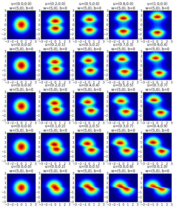
Visualizing planar flow

Visualizing the behavior of planar flow: $f(z) = z + u \tanh(w^T z + b),$ as proposed by Rezende and Mohamed, 2015.

author: Yuanjun Gao, 09/25/2016

import pandas as pd
import numpy as np

import matplotlib
import matplotlib.pylab as plt
%matplotlib inline

def h(x):
    return np.tanh(x)

def h_prime(x):
    return 1 - np.tanh(x) ** 2

def f(z, w, u, b):
    return z + np.dot(h(np.dot(z, w) + b).reshape(-1,1), u.reshape(1,-1))

plt.figure(figsize=[10,12])

id_figure = 1
for i in np.arange(5):
    for j in np.arange(5):
        theta_w = 0 #represent w and u in polar coordinate system
        rho_w = 5
        theta_u = np.pi / 8 * i
        rho_u = j / 4.0
        w = np.array([np.cos(theta_w),np.sin(theta_w)]) * rho_w
        u = np.array([np.cos(theta_u),np.sin(theta_u)]) * rho_u
        b = 0
        grid_use = np.meshgrid(np.arange(-1,1,0.001), np.arange(-1,1,0.001))
        z = np.concatenate([grid_use[0].reshape(-1,1), grid_use[1].reshape(-1,1)], axis=1)
        z = np.random.normal(size=(int(1e6),2))
        z_new = f(z, w, u, b)

        heatmap, xedges, yedges = np.histogram2d(z_new[:,0], z_new[:,1], bins=50, 
                                                 range=[[-3,3],[-3,3]])
        extent = [xedges[0], xedges[-1], yedges[0], yedges[-1]]

        plt.subplot(5,5,id_figure)
        plt.imshow(heatmap, extent=extent)
        plt.title("u=(%.1f,%.1f)"%(u[0],u[1]) + "\n" +
                  "w=(%d,%d)"%(w[0],w[1]) + ", " + "b=%d"%b)
        id_figure += 1
        
        plt.xlim([-3,3])
        plt.ylim([-3,3])

plt.savefig('planar_flow.jpg')

planar flow

References

[1] Rezende, Danilo Jimenez, and Shakir Mohamed. “Variational inference with normalizing flows.” arXiv preprint arXiv:1505.05770 (2015). link

[2] Kingma, Diederik P., Tim Salimans, and Max Welling. “Improving Variational Inference with Inverse Autoregressive Flow.” arXiv preprint arXiv:1606.04934 (2016). link

[3] Germain, Mathieu, et al. “Made: masked autoencoder for distribution estimation.” International Conference on Machine Learning. 2015.

Columbia Advanced Machine Learning Seminar

Variational Inference with Normalizing Flows

Improving Variational Inference with Inverse Autoregressive Flow

Visualizing planar flow

References