Two papers this week proved convergence results for optimizing non-convex loss functions using stochastic gradients. In The Landscape of Empirical Risk for Non-convex Losses by Mei, Song, Yu Bai, and Andrea Montanari, 2016 [1], the authors show that while empirical risk for squared loss is non-convex for linear classifiers, there are numerous desirable qualities once we reach a certain sample size, namely exponentially fast convergence to a local minimum (which is also the global minimum). In Deep Learning without Poor Local Minima by Kawaguchi (2016) [2], by reducing deep linear networks to deep nonlinear networks, the author shows that, among other things, every unique minimum is a global minimum and every non-minimum critical point is a saddle point.

The Landscape of Empirical Risk for Non-convex Losses

While non-convex optimization has historically been associated with NP-hardness, there are a plethora of non-convex functions that can be optimized more easily by taking advantage of some special structural properties. This paper focuses on the specific case of noisy linear classification, and shows that under certain assumptions, the empirical risk, which is non-convex, has a unique local minimum, which gradient descent approaches exponentially fast.

Setup

• Data is $(x_i, y_i) \in \mathcal{R}^d \times \{0, 1\}$ i.i.d.
• $P(y_i = 1 | x_i ) = \sigma(\langle w_0, x\rangle)$ for some function, $\sigma(\cdot)$, which is known.
• Loss function is empirical risk $\hat R_n(w) = \frac{1}{n}\sum_{i=1}^n (y_i - \sigma(\langle w, x_i\rangle))^2$.

We note that the empirical risk is non-convex. However, the authors argue that non-convex losses can be beneficial for this task because they are unbounded, they have a smaller number of support vectors, and models that use non-convex losses (such as neural networks) have been quite effective.

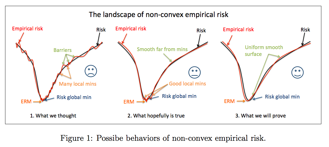
The true risk, $R(w) = \mathbb{E}((y-\sigma(\langle w, x\rangle))^2)$ is convex in terms of $w$, and the authors show that the empirical risk function ends up sharing many of these nice properties. The following graph shows three possible scenarios for the empirical risk. On the left is a function with many local minima, and in the center is a loss with local minima that are close to the risk global minimum. Niether of these are ideal, and we will see for sufficient sample data, the function behaves like the graph on the right with a local minimum that is the risk global minimum, verifying the effectiveness of stochastic gradient descent.

We make the following assumptions:

1. $\sigma$ is three times differentiable, where $\sigma'(z) > 0$ and the first three derivatives are bounded.
2. The feature vector X is sub-Gaussian, i.e. for all $\lambda \in \mathbb{R}^D$, $\mathbb{E}(e^{\langle \lambda, X \rangle}) \leq e^{\frac{\tau^2 \|\lambda\|_2^2}{2}}$.
3. $X$ spans all directions in $R^d$ so $E(XX^T) \succeq c\tau^2 I_{d \times d}$ for some $c \in (0,1)$.

Assumptions 1 and 3 appear reasonable. The assumption that deserves the most scrutiny is assumption 2, as indeed, it guides many of the proofs in the paper. We note that if $X$ is bounded, assumption 2 holds.

Results

The main result of this paper is Theorem 1 which has three parts. If $n \geq Cd \log d$ for some constant $C$,

1. $\hat R_n(w)$ has a unique local optimizer, which is also global. This implies no other critical points exist.
2. Gradient descent converges exponentially fast.
3. The global optimum of the empirical risk $\hat w_n$ converges to the true minimum $w_0$:

Looking at $n \geq Cd \log d$, $n$ is roughly the same scale as $d$, and becuase $n$ cannot be less than $d$, these results are ideal.

The authors verify these results by running experiments with simulated data and various conditions for $n$. These results verify that once $n$ crosses some critical threshold, the convergence results change dramatically.

Proof Ideas

We discuss a few theorems the authors develop to construct their proof (which is too technical to include in this writeup). The meat of their argument lies in Theorem 2, which conerns the true risk $R(w)$. Summarizing these results,

• The true risk $R(w)$ has a unique minimizer $w_0$.
• The Hessian of $R(w)$ has bounds, where in a small ball around the the global optimum, we have a strongly convex function (i.e. we converge very quickly):

• The gradient of $R(w)$ has bounds, such that when we are outside of a ball centered at the true value $w_0$, the gradients are non-zero:

Namely, this implies our gradients point toward the optimum.

The remaining theorems in the paper bound the probabilities that the gradient and Hessian of empirical risk differ from the true risk by a constant. Combining these probabilities with Theorem 2, the authors conclude that the desirable qualities are recovered with a high probability when using the non-convex empirical risk, as opposed to true risk.

Discussion

We were curious whether the proofs can generalize to functions beyond squared loss, since in real life squared-loss isn’t the most frequently used loss for classification.

Overall, we thought this was a very well-written paper that did a good job of stating the high-level at the beginning, while exploring the technical details throughout.

Deep Learning without Poor Local Minima

The key assumption of this paper is that, under certain conditions, deep linear neural networks are similar to deep nonlinear neural networks. The author proves four optimization results for deep linear neural networks, and via a reduction, shows that these extend to nonlinear neural networks.

Setup

Our data is of the form $(X, Y)$, where, for some weight parameters $W$ and a nonlinearity $\sigma(\cdot)$, our predictions for a nonlinear network take the following form:

We use squared loss: $L = \frac{1}{2} \| \hat Y(W,X) - Y \|^2_F$, where $\|\cdot \|_F$ is the Frobenius norm. It has been proven that this optimization is NP-hard. However, for now, let’s assume a deep linear network. That is, $\sigma(\cdot) = 1$, so

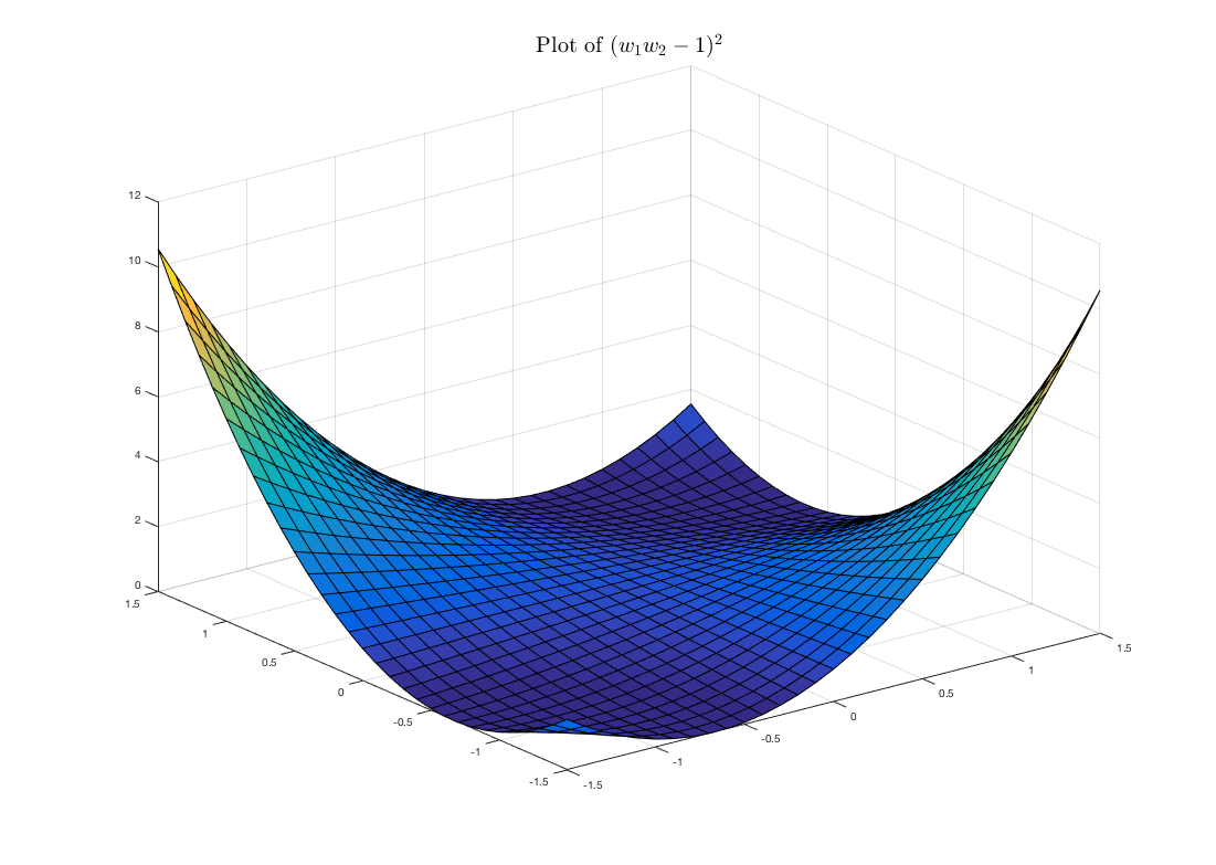
The author shows that this function is non-convex in the product of the weight matrices. As an example, take the simplest case, where $X = Y = 1$, and we have weight scalars $w_1$ and $w_2$. The plot below depicts our loss function $(w_1w_2-1)^2$. As we can see, even in the simplest case, there are infinite global minima when $w_1 = \frac{1}{w_2}$, in addition to saddle points.

Results

The main result for deep linear networks is in Theorem 2.3. Here, under reasonable assumptions for the rank of our data, for any depth $H \geq 1$ and $p$ the smallest width of a hidden layer, the loss function $L(W)$ has the following properties:

1. It is non-convex and non-concave.
2. Every local optimum is global.
3. Every critical point that is not a global minimum is a saddle point.
4. If Rank($W_H \cdots W_2)= p$, then the Hessian at a saddle point has at least one negative eigenvalue.

We note that a Hessian having at least one negative eigenvalue is “nice”, in that it implies there are no flat regions in the function. Briefly, the proof ideas are as follows. For 1, if we set one $W$ entry to 0, the product is fixed at 0, meaning that the function doesn’t change in $W$, implying non-convexity. For 2, we rely on the notion of a “certificate of optimality”; that is, we check that at every local minimum, $0 = X(X^TW^T-Y^T)$, implying the local optimum is global. 3 follows naturally from 2, and 4 is somewhat technical. For the full proofs, refer to the original paper [2].

We next focus on a reduction from nonlinear neural networks to linear neural networks. Here, we take $\sigma(\cdot)$ as the hinge loss, i.e. $\sigma(b) = \max(b, 0)$. Taking advantage of a neural network’s graphical strucutre, the author notes we can rewrite the objective by summing over all possible paths, introducing a binary random variable $Z_i$ to denote those that are turned “on” by the activation function. Specifically, we can write the following, where $q$ is a normalization constant and $\Psi$ is the toal number of paths from the inputs to each output:

Now, we introduce the central assumption of the paper: Each $Z$ is independent of $X$, and is a Bernoulli random variable with a global probability $p$. Thus, replacing the $Z_i$ with $p$ in the above equation reduces this loss to that of a deep linear neural network, so all the results from Theorem 2.3 hold.

We spent a lot of time discussing how realistic this claim is. We note that it improves upon previous work, which had stronger assumptions and proved weaker results. However, it appears suspicious that all the $Z_i$ are i.i.d. random variables, and this claim should receive scrutiny.

All-in all, we thought this was a well-organized paper that outlined intuitive and important theoretical results for deep neural networks.

References

[1] Mei, Song, Yu Bai, and Andrea Montanari. “The Landscape of Empirical Risk for Non-convex Losses.” arXiv preprint arXiv:1607.06534 (2016). link

[2] Kawaguchi, Kenji. “Deep Learning without Poor Local Minima” arXiv preprint arXiv:1605.07110 (2016). link …