This week, we read Gal and Ghahramani’s “Dropout as a Bayesian Approximation: Representing Model Uncertainty in Deep Learning” [1], as well as “Deep Networks with Stochastic Depth” by Huang et. al [2]. The two papers differed greatly in scope: Gal and Ghahramani looked at Dropout from a Bayesian point of view and cast it as approximate Bayesian inference in deep Gaussian Processes while Huang et al. demonstrated the possibility of incorporating Dropout in the Resnet architecture.

The figures and tables below are taken from the aforementioned papers.

Dropout as a Bayesian Approximation: Representing Model Uncertainty in Deep Learning

Generally, standard deep learning tools for regression and classification do not capture model uncertainty. But having estimates of model uncertainty is important when deploying deep learning and deep reinforcement models as given such estimates, we would be able to treat uncertain inputs and special cases with greater care in the former and learn faster in the latter. Here, Gal and Ghahramani show that Dropout can be understood as approximate Bayesian inference in deep Gaussian Processes and hence model uncertainty can be captured under the Bayesian framework.

Setup

• Observed inputs $x = \{x_i\}_{i=1}^N$ and outputs $y = \{y_i\}_{i=1}^N$
• Set of model parameters $\omega$
• Define prior distribution over $\omega$ as $p(\omega)$ and likelihood as $p(y \mid \omega, x)$
• We want to find the posterior $p(\omega \mid y, x)$

Moving to the Bayesian neural networks world, we define the weights $w$ and bias $b$ to be part of the model parameters $\omega$ but in this analysis we omit $b$ for simplicity. For the weights $w_{\ell, \ell-1}$ linking the $\ell$ and $\ell -1$ layers: we represent it as matrix of dimension $K_{\ell} \times K_{\ell - 1}$ where $K_{\ell}$ is the number of nodes in the $\ell^{th}$ layer. With this in place, set a prior $p(w_{ik}) \propto \exp\{-\frac{1}{2}w_{ik}^T w_{ik}\}$ for layer $i$ and column $k$. We now have $y = f(x, \omega) = w_L \sigma(... w_2 \sigma(w_1 x)...)$.

Here, we use the commonly defined loss function for dropout

Variational Inference

We use variational inference to approximate the posterior $p(\omega \mid x, y)$ with $q_\theta(\omega)$. Our loss function $\mathcal{L}(\theta)$ is then in the form of

and the first term can be approximated by MCMC integration which gives an unbiased estimator. Define the approximated $\mathcal{L}(\theta)$ as $\hat{\mathcal{L}}(\theta)$.

Moving on to $q_\theta(\omega)$, given variational parameters $\theta = \{m_{ik}\}_{i,k}$ we set our approximate posterior as

where $q_{m_ik}(w_{ik}) = p_i \delta_0(w_{ik}) + (1 -p_i)\delta_{m_{ik}}(w_{ik})$. As we are working in continous space, we approximate the $\delta$ functions with $\mathcal{N}(0, \sigma^2)$ where $\sigma^2 \rightarrow 0$.

We can also look at this in terms of a generative process.

For every round of minimisation:

• Sample $z_{ik} \sim \mathrm{Bernoulli}(p_i)$ for each layer $i$ and column $k$
• Set $w_{\ell, \ell -1} := w_{\ell, \ell -1} \cdot \text{diag}([z_{ik}]_{k=1}^k]$). Note that this sets columns of $w_{\ell, \ell -1}$ to $0$, which is equivalent to dropping out the $j^{th}$ unit in the $i^{th}$ layer
• Minimise $\hat{\mathcal{L}}(\theta)$ w.r.t to $\theta = \{m_{ik}\}_{i, k}$

With the above in place, we now approximate the $\mathrm{KL}$ term within $\hat{\mathcal{L}}(\theta)$ as $\frac{1}{2} \sum_{LK} m_{ik}^2 + C$ (see the appendix [3] for proof). Putting it all together, we have

which looks exactly like $\mathcal{L}_{dropout}$.

After obtaining the posterior, we can estimate the approximate predictive distribution $p(y^* \mid x) = \int p(y^* \mid \omega, x) q_\theta(\omega) \mathrm{d}\omega$ using Monte Carlo methods.

Results and Discussion

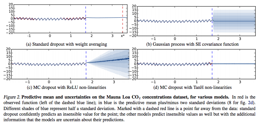
The following figure demonstrates the uncertainty estimates produced by the approximate posterior distribution

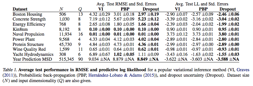
and the table below shows that the above method leads to superior predictive performance on almost every dataset

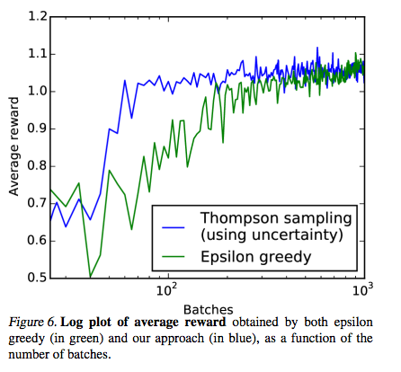
Lastly, this figure shows the speed up in learning rate for reinforcement learning

The authors postulated that the improved results was due to the model fitting the distribution that generated the observed data and not just its mean and remarked that the many Bernoulli draws in $q_\theta(\cdot)$ was a cheap way of obtaining a multi-modal posterior.

Deep Networks with Stochastic Depth

The premise of Huang et. al’s paper was to address the problems of training very deep networks: vanishing gradients, dimnished forward flow and long training times. Essentially, in the case of of Resnets, the authors demonstrate that dropping out entire layers to train short networks and using deep networks at test time leads to state-of-the-art results in most image datasets.

ResNet Primer

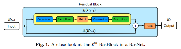
Resnets are composed of $L$ residual blocks (ResBlocks) with blocks having the update rule $H_\ell = \mathrm{ReLU}(f_\ell(H_{\ell-1}) + id(H_{\ell-1})$. The above figure shows a schemantical representation of a block with $f_\ell$ defined as a sequence of Conv(olution)-B(atch)N(ormalisation), or ReLu-Conv-BN layers. Such a scheme was used in all experiments in the paper.

Stochastic Depth

The gist of stochastic depth is to shrink the depth of a network during training and keep it unchaged during testing. This is done by skipping out entire ResBlocks during training using skip connections. Define $b_\ell \in \{0, 1\}$ as Bernoulli r.v. indicating that the $\ell$-th ResBlock is active ($b_\ell = 1$) and inactive ($b_\ell = 0$) and the survival proability as $p_\ell = P(b_\ell = 1)$. By multiplying $f_\ell(H_{\ell-1})$ by $b_\ell$, we can drop the whole block out if $b_\ell$ is set to $0$, which results in

In this setting, we have $p_\ell$ as a new hyperparameter. As earlier layers extract low-level features and should be present most of the time, a simple linear rule from $p_0 = 1$ for the input to $p_L$ for the last ResBlock is

This modification reduces the depth of the network as the expected network depth is $\mathbb{E}(L) = \sum_L p_\ell$, which also results in training time savings. Huang et. al also characterise the different sets of ResBlock for each minibatch as an implicit ensemble of ResBlock within the ResNet itself and postulates that such a configuration gives rise to better results. However, we are not very convinced by this claim based on what we know in classical ML.

During test time, the forward propagation update rule is

to account for the probability of each layer “surviving”.

Results

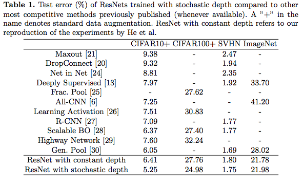
The table below shows that ResNets with stochastic depth tends to outperform other architectures on most image datasets apart from ImageNet

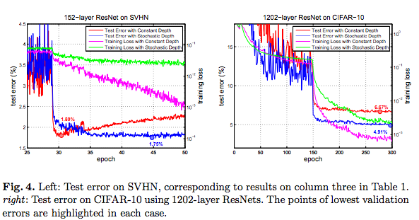
and following figure demonstrates that stochastic depth prevents overfitting in 1202-layer ResNet, giving rise to a network of more than 1000 layers further reducing the test error on the CIFAR-10 dataset.

[1] Gal, Y. and Ghahramani, Z., 2015. Dropout as a Bayesian approximation: Representing model uncertainty in deep learning. arXiv preprint arXiv:1506.02142. link

[2] Huang, G., Sun, Y., Liu, Z., Sedra, D. and Weinberger, K., 2016. Deep networks with stochastic depth. arXiv preprint arXiv:1603.09382. link

[3] Gal, Y. and Ghahramani, Z., 2015. Dropout as a Bayesian approximation: Appendix. link