This week we read and discussed two papers: a paper by Johnson et al. [1] titled “Composing graphical models with neural networks for structured representations and fast inference” and a paper by Gao et al. [2] titled “Linear dynamical neural population models through nonlinear embeddings.” Although the two papers have different focuses — the former proposes a general modeling and inference framework, whereas the latter focuses in particular on modeling neural activity — they are similar in that both use structured latent variable models as part of a variational autoencoder framework in order to perform inference. The benefit to this type of approach is that it allows for an increase in the flexibility of the models we can consider while retaining interpretability, even in high dimensions.

The figures and algorithms below are taken from the aforementioned papers.

SVAE — Structured Variational Autoencoders

We first discussed the paper of Johnson et al [1], which combined ideas from probabilistic graphical models and deep learning in order to propose a joint modeling and inference framework, which attempts to allow for flexible and interpretable representations of complex high dimensional data. Generally, probabilistic graphical models provide structured representations which are frequently inflexible, whereas (for example) variational autoencoders are able to learn flexible data representations but may not encode an interpretable probabilistic structure. Ideally, we would like to be able to combine the strengths of these two approaches and eliminate the weaknesses.

The general framework proposed by the paper in order to achieve this, which they refer to as the structured variational autoencoder (SVAE), can be broadly motivated as follows. In an exponential family latent variable model, we have efficient inference algorithms for when the observation model is conjugate; however, these algorithms depend on structures which break down when we do not have conjugacy. One particular way of handling non-conjugate observation models is by using the variational autoencoder, which introduces recognition networks in order to do so. The main idea of the SVAE is therefore to learn recognition networks that output conjugate graphical model potentials, so that they can be used in graphical model inference algorithms as a surrogate for the (non-conjugate) observation likelihood.

Notation and setup

Here we denote $\theta$ as our global latent variables and $x = \{x_n\}_{n=1}^N$ as our local latent variables. We then let $p(x|\theta)$ be an exponential family and $p(\theta)$ the corresponding conjugate, so

where by conjugacy we may write $t_{\theta}(\theta) = \left( \eta^0_x(\theta), - \log Z_x(\eta^0_x(\theta)) \right)$. We then denote our general observation model for the data as $p(y|x, \gamma)$ (for example, this may be obtained via some neural network) and let $p(\gamma)$ be a exponential family prior on $\gamma$. The aim is to then obtain (an estimate for) the posterior $p(\theta, x, \gamma | y)$.

Variational inference

Fixing $y$, we can consider the mean field family $q(\theta)q(\gamma)q(x)$ and the variational inference objective

in order to approximate the posterior. The authors then make some further restrictions:

• $q(\theta)$ is restricted to belong to the same exponential family as $p(\theta)$ with natural parameters $\eta_{\theta}$,
• $q(\gamma)$ is restricted to belong to the same exponential family as $p(\gamma)$ with natural parameters $\eta_{\gamma}$
• $q(x)$ is restricted to belong to the same exponential family as $p(x \mid \theta)$ with natural parameters $\eta_{x}$

and denote the above variational inference objective as $\mathcal{L}(\eta_{\theta}, \eta_{\gamma}, \eta_x)$.

To efficiently optimize over this objective, one approach is to consider $\eta_x$ as a function of the other parameters. As $p(y | x, \gamma)$ may generally be intractable, this term in the objective is replaced by a term conjugate to the exponential family $p(x| \theta)$, and so $\eta_x$ is now selected by optimizing over a surrogate objective

where $\psi(x; y, \phi) := \langle r(y;\phi), t_x(x) \rangle$ and $\{ r(y;\phi) \}_{\phi \in \mathbb{R}^m}$ is a parameterized class of functions corresponding to the recognition model. Defining

one can show that the corresponding factor $q^*(x)$ is given by

Although $q^*(x)$ is suboptimal for $\mathcal{L}$, this factor is at least tractable to compute.

The SVAE objective

The SVAE objective is then defined as

and it is this objective which the SVAE algorithm attempts to maximize. Proposition 4.1 of the paper shows that the SVAE objective is a lower bound for the mean field objective for any recognition model $\{ r(y; \phi) \}_{\phi \in \mathbb{R}^m}$; to provide the best lower bound, we will want to choose this class to be as large as possible.

The approach of first optimizing for $\eta_x$ as a local partial optima of $\hat{\mathcal{L}}$ has two computational advantages; firstly, by exploiting the graphical model structure, $\eta^*_x$ and expectations with respect to $q^*(x)$ are quick to compute. Secondly, the natural gradient can be easily estimated; without going into the finer details, the natural gradient for SVAE is a sum of a the natural gradient in SVI, plus a term which is estimated as part of computing the gradients with respect to the remaining parameters.

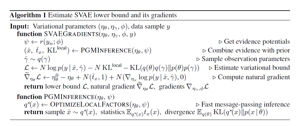
For sake of completeness, the SVAE algorithm is reproduced below:

Experiments

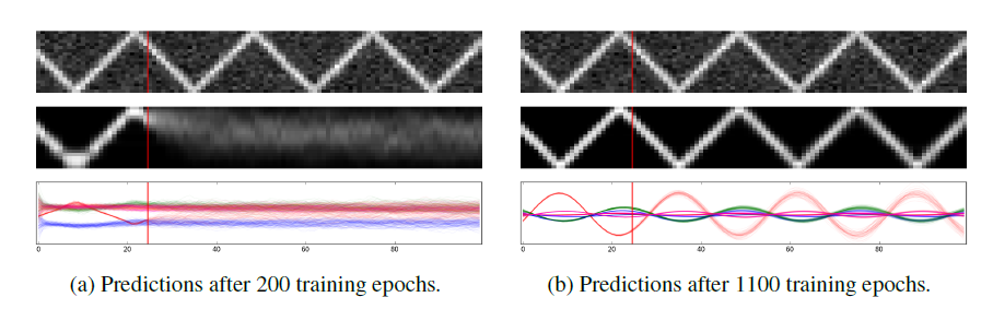
In the paper SVAE is applied to a variety of synthetic and real data; we briefly highlight one of their experiments. Here, they use a latent linear dynamical system (LDS) SVAE to model a sequence of one dimensional images representing a dot bouncing from top to bottom of the image. The below figure shows the results from prediction at different stages of training; the top panel an example data sequence, the middle the (noiseless) predictions from the SVAE, the bottom the corresponding latent states, and the vertical line representing the training data. We can see that the algorithm is able to represent the image accurately (after sufficiently many training epochs).

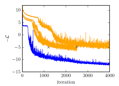
More importantly, this experiment illustrates how the natural gradient algorithm learns more quickly than that standard gradient descent, while also being less dependent on the parameterization. This can be seen in the figure below, which shows how $-\mathcal{L}$ evolves with iteration number when using natural (blue) and standard (orange) gradient updates (where X’s mark early termination), for three different learning rates.

fLDS - Linear dynamical systems with non-linear observations

We then discussed the paper by Gao et al. [2], which is similar to the first paper in that a latent variable approach is used, but here the authors focus on one problem — that of modeling firing rates of neurons. Here this is done by modeling these rates as an arbitrary smooth function of a latent, linear dynamical state. As in the SVAE paper, the aim is to allow for more modeling flexibility (in this case, that of neural variability) while retaining interpretability, which in this case corresponds to having a low-dimensional, visualizable latent space, even though the actual neural data is high-dimensional and non-linear.

Neural data and notation

In neural data, signals take the form of $\sim 1$ms spikes that are modeled as discrete events. For data analysis, time is discretized into small bins of length $\delta t$, and the response of a population of $n$ neurons at time $t$ is represented by a vector $x_t$ of length $n$. As spike responses are variable under identical experimental conditions, usually many repeated trials, $r \in \{1, \ldots, R\}$, of the same experiment are recorded. We therefore denote

as spike counts of $n$ neurons for time $t$ and trial $r$. We then also refer to $x_r = (x_{r1}, \ldots, x_{rn}) \in \mathbb{N}^{T \times n}$ when suppressing the time index, and $x = (x_1, \ldots, x_R) \in \mathbb{N}^{T \times n \times R}$ to denote all the observations. Similar notation is used for other temporal variables.

fLDS generative models

Latent factor models are commonly used in neural data analysis, and attempt to infer latent trajectories $z_{rt} \in \mathbb{R}^m$ which are low-dimensional ($m \ll n$) and evolve in time. One approach takes inspiration from the Kalman filter, so that the latent states evolve according to

where $A \in \mathbb{R}^{m \times m}$, and $Q_1, Q$ are covariance matrices. In fLDS, the observation model is given by

where

• $\mathcal{P}_{\lambda}(\lambda)$ is a noise model with parameter $\lambda$,
• $f_{\psi} : \mathbb{R}^m \to \mathbb{R}^n$ is an arbitrary continuous function.

Here, $f_{\psi}(\cdot)$ is represented through a feed-forward neural network model, so the parameters $\psi$ amount to weights/biases across units and layers. The aim is to then learn all the generative model parameters, which are denoted by $\theta$.

Fitting via Auto-encoding Variational Bayes (AEVB)

Due to the noise model and the non-linear observation model, the posterior $p_{\theta}(z | x)$ is intractable and so the authors employ a stochastic variational inference approach. The posterior is then approximated by a tractable distribution $q_{\phi}(z | x)$ depending on parameters $\phi$ and the corresponding evidence lower bound $\mathcal{L}$ (ELBO) is maximized; here, an auto-encoding variational Bayes approach is used to estimate $\nabla \mathcal{L}$. Given these, the ELBO is then maximized via stochastic gradient ascent.

This approach ends up being similar to that of the first paper, when considering the choice of approximate posterior distributions used. Here, a Gaussian approximation is used:

where $\mu_{\phi}(x_r)$ and $\Sigma_{\phi}(x_r)$ are parameterized by the observations through a structured neural network. This idea is similar to that in the SVAE paper, where we approximate the observation model by an exponential family conjugate to the model for the local latent variables with a diverse class of potential functions; here, we approximate the posterior for the latent variables by the conjugate family to that of the prior with a similarly diverse class of potential functions.

Experiments

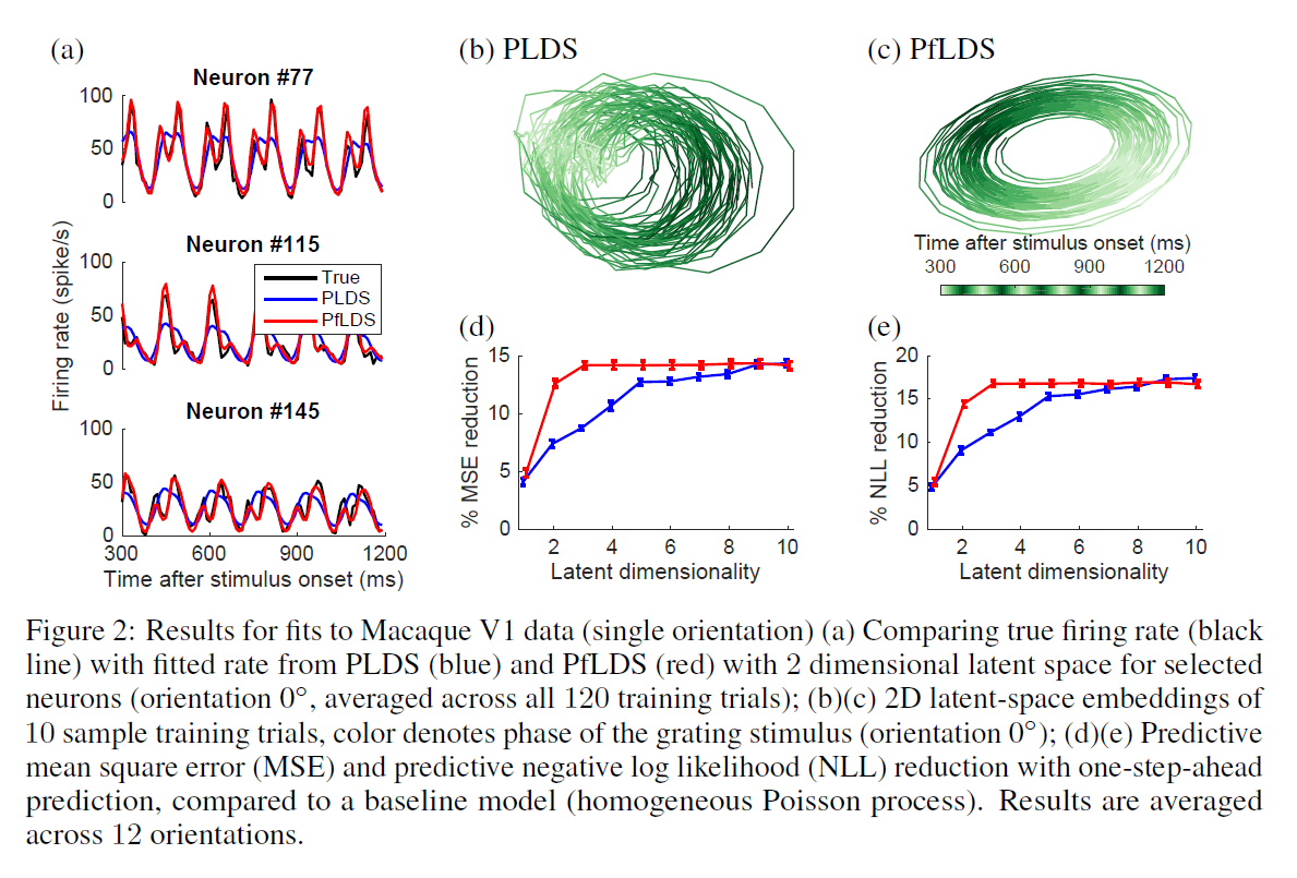
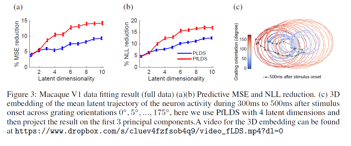
The above model is applied to various simulation and real data; we briefly describe one of the real data examples provided in the paper. Here, they look at neural data obtained from an anesthetized macaque, which was taken while the monkey watched a movie of a sinusoidal grating drifting in one of 72 orientations (starting from 0 degrees and incrementing in 5 degree steps). They then compare PfLDS (a fLDS with Poisson noise model) with a PLDS (Poisson LDS) using both a single orientation (0 degrees) and the full data, using a fraction of the data for training before assessing model fitting by one-step-ahead prediction on a held-out dataset. The figure below illustrates the performance of the two models when looking at single-orientation data; we can see that PLDS requires 10 latent dimensions to obtain the same predictive performance as a PfLDS with 3 latent dimensions - the PfLDS leads to more interpretable latent-variable representations.

For the full orientation data, the below figure illustrates this principle again - that it provides better predictive performance with a small number of latent dimensions.

References

[1] Johnson, Matthew J., et al. “Composing graphical models with neural networks for structured representations and fast inference.” Advances in Neural Information Processing Systems (2016). link

[2] Gao, Yuanjun, et al. “Linear dynamical neural population models through nonlinear embeddings.” Advances in Neural Information Processing Systems (2016). link