In this week’s session we read and discussed two papers relating to GANs: Wasserstein GAN (Arjovsky et al. 2017 [1]) and Adversarial Variatonal Bayes: Unifying Variational Autoencoders and Generative Adversarial Networks (Mescheder et al. 2017 [4]). The first paper introduces the use of the Wasserstein distance rather than KL divergence for optimization in order to counter some of the problems faced in original GANs. The second paper synthesizes GANs with VAEs in an effort to allow arbitrarily complex inference models.

The figures and tables below are copied from the aforementioned papers.

Review of GANs

GANs were introduced by Goodfellow et al. in 2014 [2] as an alternative to the maximum likelihood approach to generative models. In a maximum likelihood framework, we define a distribution $x_i \sim p_\theta$ over our data $\{x_i\}_{i=1}^n$ and choose parameters $\theta$ such that the likelihood of the training data is maximized: $\theta^*={\text{argmax}_{\theta}} \prod_{i=1}^n p_\theta(x_i)$.

In a GAN framework, the problem is formulated as a minimax game between a generator function G, and a discriminator function D. The classic analogy for this is that of a counterfeiter and a policeman. The policeman (D) tries to maximize his ability to distinguish between counterfeit products and real products, while the counterfeiter (G) simultaneously tries to produce material that is as close to the real deal as possible.

Define the following notation:

• $p_\mathcal{D}$ - the true data generating distribution
• $p_z$ - prior on the latent variables $z$
• $p_g$ - the distribution over fake generated data, $D(G(z))$

Setting this up as a minimax game, D is trained to maximize the probability of assigning $x$ to the real data rather than the generated data $p_g$, while G is trained to minimize the discrepancy between the real data and the generated data. The value function is given by:

To optimize this, the following updates are used:

• (D) Discriminator

• (G) Generator

The optimal discriminator for any generator can be shown to be: $D^* = \frac{p_\mathcal{D}}{p_\mathcal{D}+p_g}$ [2]. Plugging this in to the value function for the game,

where JS is the Jenson-Shannon divergence.

Problems with GANs

• Unstable training: It is hard to balance between optimizing G and D
• Collapse of the mode, also called mode dropping
• High dependency on the architecture of the NN
• Hard to quantify how well a model does outside of an arbitrary “these generated pictures look good”

Wasserstein GAN

This paper overcomes some of the problems with the original GANs through the introduction of an alternative metric to KL divergence. When looking at distributions over low dimensional manifolds, the chance of their having overlapping support is low, resulting in an undefined or infinite KL divergence. The Earth-Mover, or Wasserstein-1, distance is defined as the cost of the optimal transport plan:

The name “Earth-Mover” can be understood by thinking of each distribution as a pile of dirt, with the EM distance defined as the amount of dirt that needs to be moved times the distance it needs to be moved.

In Example 1 of [1], this paper presents two distributions with a negligible intersection in order to highlight the problems that arise when using KL and JS divergence. Take $Z \sim U[0,1]$ and define $\mathbb{P}_0$ to be the distribution of $(0,Z)\in\mathbb{R}^2$. Let $\mathbb{P}_\theta$ be the distribution of $(\theta, Z)$. Some commonly chosen metrics in this case are:

• Wasserstein or “Earth-Mover”: $W(\mathbb{P}_0, \mathbb{P}_\theta) = |\theta|$
• Jensen-Shannon: $JS(\mathbb{P}_0, \mathbb{P}_\theta) = \log 2$ if $\theta \neq 0$, $0$ otherwise
• Kulback-Leibler: $KL(\mathbb{P}_\theta \| \mathbb{P}_0) = + \infty$ if $\theta \neq 0$, $0$ otherwise

As $\theta \to 0$, $\mathbb{P}_\theta$ converges to $\mathbb{P}_0$ under the EM distance, but not under the JS or KL distances. The JS and KL distances are not even continuous in this instance. The authors formalize this idea in in Theorem 1 [1], providing continuity results for the EM distance that motivate the choice of using this as a loss function.

To optimize over $W(p_\mathcal{D}, p_g)$ instead of $JS(p_\mathcal{D}, p_g)$, something must be done about the intractable infimum present in the definition of Wasserstein distance. Enter the handy Kantorovich-Rubinstein duality. Using this duality, the EM distance can be reformulated as $W(p_\mathcal{D}, p_g) = \sup_{\|f\|_L \leq 1} \; \mathbb{E}_{x\sim p_\mathcal{D}}[f(x)]-\mathbb{E}_{x\sim p_g}[f(x)]$, where the supremum is over all 1-Lipschitz functions.

The Wasserstein GAN (WGAN) is then optimized through the following updates:

• (D) $\max_{w \in \mathcal{W}} \; \mathbb{E}_{x\sim p_\mathcal{D}} f_w(x)-\mathbb{E}_{z\sim p(z)}f_w(g_\theta(z))$
• (G) $\min_{\theta} \; \mathbb{E}_{z \sim p_z} f_w(g_\theta(z))$ where $w \in \mathcal{W}$ are weights that parameterize a neural network. To ensure $w$ lie in a compact space, the weights are clamped to $\mathcal{W} = [-c,c]^l$.

Solving this optimization problem is done through the algorithm described below:

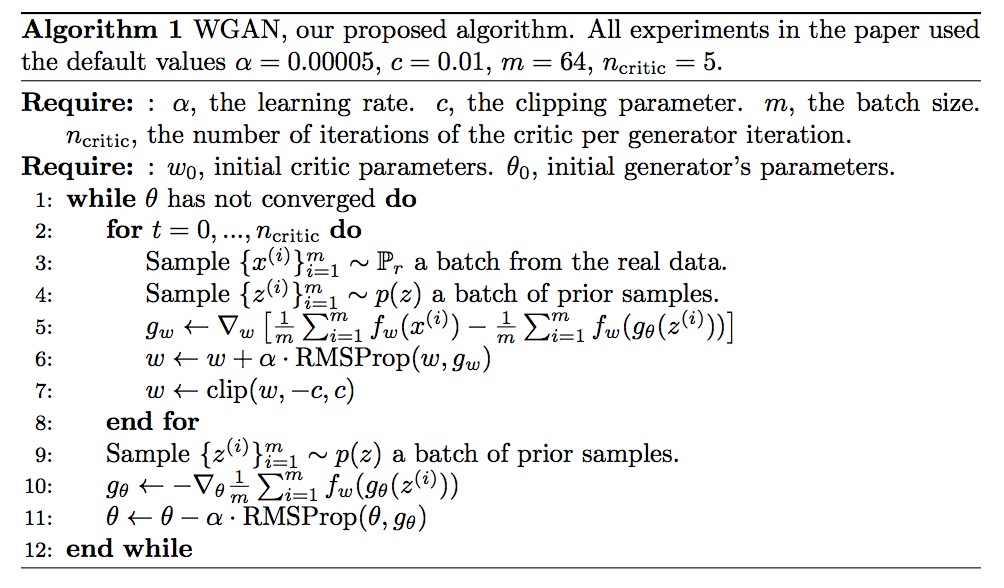
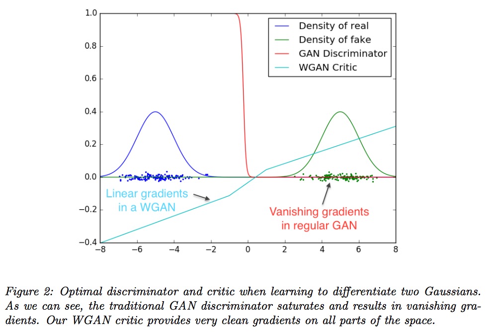
The weight constraint prevents the discriminator from saturating by limiting D to grow at most linearly. The continuity and differentiability of the EM distance allows D to be trained to optimality, preventing the modes from collapsing as before.

In the experiments section, the authors confirm their assertions, even bringing out the bold font in Section 4.3 to emphasize their circumvention of mode collapsing. It is also important to note that the nonstationarity of D results in a worse performance for momentum based methods like Adam, causing them to use RMSProp instead.

Adversarial Variational Bayes

This paper presents an adversarial procedure for training Variational Autoencoders ([3]) that uses the flexibility of neural networks to allow arbitrarily complex inference models.

Review of VAEs

Consider data $\{ x_i\}_{i=1}^n$ generated from some distribution $p_\theta(x \mid z)$ over latent continuous variables $z \sim p(z)$. We are interested in the true posterior density $p_\theta(z \mid x)$. This distribution is often intractable, and so we approximate it with an approximate inference model, $q_\phi(z\mid x)$. We wish to choose the model $q$ that minimizes the KL divergence between the approximate posterior and the true posterior:

A common result in variational inference bounds the marginal likelihood of $x$ by the variational lower bound (or ELBO):

This lower bound is used to define the objective function we wish to optimize:

AVB

This paper starts by rewriting the objective function in the following form:

Ideally, we want $q_\phi(z\mid x)$ to be arbitrarily complex. But if $q_\phi(z\mid x)$ is defined through a black-box procedure, it can no longer be optimized using the reparameterization trick and stochastic gradient descent, as in the VAE set-up [3]. To get around this, the authors define a discriminative network $T(x,z) = \log p(z) - \log q_\phi(z \mid x)$ that is optimized simultaneously.

The objective function for $T$ is as follows:

where $\sigma(T)$ is the sigmoid function. In this way $T$ is optimized to distinguish between pairs $(x,z)$ sampled independently from $p_D(x)p(z)$ and those sampled from the current model $p_D(x)q_\phi(z\mid x)$. The optimal discriminator for this objective is shown to be $T^* = \log q_\phi(z\mid x)-\log p(z)$. The new objective function is then,

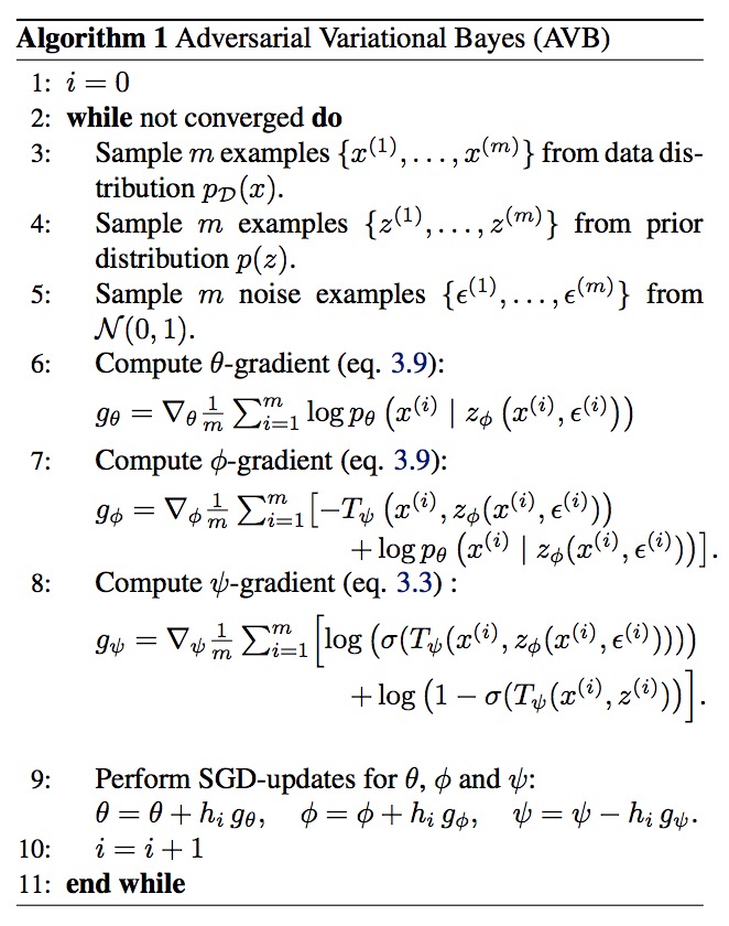
In Proposition 2, the authors show that the gradient of $T^*$ with respect to $\phi$ satisfies $\mathbb{E}_{q_\phi} \nabla_\phi T^*(x,z) = 0$. Therefore, taking the gradients with respect to $\theta$ and $\phi$ is straightforward. Using the reparameterization trick of [3], the AVB algorithm alternates between optimizing the objective function and the discriminative network $T$:

As in the original GAN setup, the optimal discriminator can be shown to be: $\sigma(T^*) = \frac{q_\phi(z \mid x)}{q_\phi(z\mid x) + p(z)}$. By allowing $T$ and $q_\phi(z\mid x)$ to be arbitrarily complex, Corollary 4 proves that the game will recover the ML estimate $\theta^*$. Additionally, Corollary 4 proves that $T^*(x,z) = \log \frac{p_{\theta^*}(x,z)}{p_{\theta^*}(x)p(z)}$ is the pointwise mutual information between $x$ and $z$.

The experiments indicate an improvement between VAE and AVB on a variety of generative tasks. Their performance on a toy example is seen below:

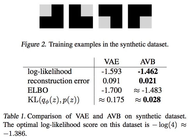
For a nice implementation of this example, see here.

References

[1] Arjovksy, et al. “Wasserstein GAN.” arXiv preprint arXiv:1701.07875 (2017). link

[2] Goodfellow, et al. “Generative Adversarial Networks.” Advances in Neural Information Processing Systems (2014). link

[3] Kingma, et al. “Auto-Encoding Variational Bayes.” International Conference on Learning Representations (2014). link

[4] Mescheder, et al. “Adversarial Variational Bayes: Unifying Variational Autoencoders and Generative Adversarial Networks.” arXiv preprint arXiv:1701.04722 (2017). link