This post begins with an apparent contradiction: on the one hand, the reparameterization trick seems limited to a handful of distributions; on the other, every random variable we simulate on our computers is ultimately a reparameterization of a bunch of uniforms. So what gives? Our investigation into this question led to the paper, “Reparameterization Gradients through Acceptance-Rejection Sampling Algorithms,” which we recently presented at AISTATS [1]. In it, we debunk the myth that the gamma distribution and all the distributions that are derived from it (Dirichlet, beta, Student’s t, etc.) are not amenable to reparameterization [2-5]. We’ll show how these distributions can be incorporated into automatic variational inference algorithms with just a few lines of Python.

Shortcuts

If you’ve got the basics down, feel free to skip to the new stuff!

For code, skip to the end. Note: the code will make a lot more sense after going through this post.

Here’s the paper info:

Naesseth, Christian, Francisco Ruiz, Scott Linderman, and David Blei. “Reparameterization Gradients through Acceptance-Rejection Sampling Algorithms.” Artificial Intelligence and Statistics (AISTATS). 2017. link

Background

If the intro didn’t make any sense, never fear. We’ll start with the basics of variational inference, reparameterization and score function gradients, and rejection sampling. Then we’ll show how to combine these ideas to develop general purpose variational inference algorithms for a broad class of variational distributions, namely, those that can be sampled via rejection sampling. Finally, we’ll show that it works! Across a variety of examples, our rejection sampling variational inference algorithm leads to faster convergence of the variational lower bound.

Variational Inference and the ELBO

Variational Bayesian inference, like all approximate Bayesian inference, is about estimating the posterior distribution of some latent variables given observed data,

$p(z \mid x) = \frac{p(x, z)}{\int p(x, z) \, \mathrm{d}z}.$

Of course, if we don’t assume any special model structure, the integral on the right hand side will generally be intractable and we’ll have to resort to approximate methods. Variational inference is one such method, and it’s based on the following idea: we should recast this integration problem as an optimization problem. We start by specifying a family of “nice” densities $\mathcal{Q}$ . Each member of this family will be a density $q(z; \theta)$ indexed by parameter $\theta$ . What does “nice” mean? Roughly, we should be able to evaluate the densities (including their normalization constant) and draw samples from them. Our goal is to find the parameters $\theta^*$ such that $q(z; \theta^*)$ best approximates the true posterior, $p(z \mid x)$ .

Approximation accuracy is typically measured by the Kullback-Leibler (KL) divergence from $q$ to $p$ . With a bit of algebra, we can show that minimizing the KL divergence is equivalent to maximizing the “evidence lower bound,” or ELBO,

$\mathcal{L}(\theta) = \, \mathbb{E}_{q(z; \theta)} \left[\log p(x, z) \right] + \mathbb{H}\left[q(z; \theta) \right].$

where $\mathbb{H}[q(z; \theta)]$ is the entropy of $q(z; \theta)$ .

How do we optimize the ELBO? It turns out that stochastic gradient ascent often works pretty well. We just need (an unbiased estimate of) the gradient, $\nabla_\theta \mathcal{L}$ . This is where the reparameterization trick comes in.

Reparameterization vs Score Function Gradients

For now, let’s assume the entropy of $q$ is tractable. Still, the expectation in the ELBO is another high dimensional integration problem, and this integral cannot be computed in closed form, by assumption. Fortunately, we can still compute Monte Carlo estimates of the gradient, effectively swapping the order of integration and differentiation. There are two main ways of doing this.

The first method is the score function gradient, a.k.a. the REINFORCE gradient, which we estimate with Monte Carlo $^1$ :

$\nabla_\theta \mathbb{E}_{q(z; \theta)} [\log p(x, z)] = \, \mathbb{E}_{q(z; \theta)} [\log p(x, z) \nabla_\theta \log q(z; \theta)],$

While the score function gradient is broadly applicable to nearly any variational distribution, regardless of whether $z$ is discrete or continuous, it tends to yield high variance estimates. In practice, the score function gradient must be combined with control variates and other variance reduction methods [6]. Even with these techniques, score function gradients can still be too high variance to converge in a reasonable amount of time.

If we are willing to sacrifice some amount of flexibility, we can obtain much lower variance gradient estimates using the reparameterization trick. Suppose $z$ is a continuous random variable that can be simulated by a simple transformation $z=h(\epsilon; \theta)$ with $\epsilon \sim s(\epsilon)$ . Here, $\epsilon$ is another random variable whose density is independent of the parameters $\theta$ , and $h$ is a differentiable function. For example, $q(z; \theta) = \mathcal{N}(z \mid \theta, 1)$ can be reparameterized as $z = \theta + \epsilon$ where $s(\epsilon) = \mathcal{N}(\epsilon \mid 0,1)$ . In such cases,

$\nabla_\theta \mathbb{E}_{q(z; \theta)} [\log p(x, z)] = \, \mathbb{E}_{s(\epsilon)} \left[ \nabla_\theta \log p(x, h(\epsilon; \theta)) \right]$

After reformulating the problem as an expectation with respect to $s(\epsilon)$ , we can (under mild assumptions that we’ll get to shortly) swap the order of integration and differentiation. This technique tends to yield low variance Monte Carlo estimates of the gradient, but it is limited in scope: we need $z$ to be a continuous random variable and $h$ to be differentiable.

Rejection Sampling

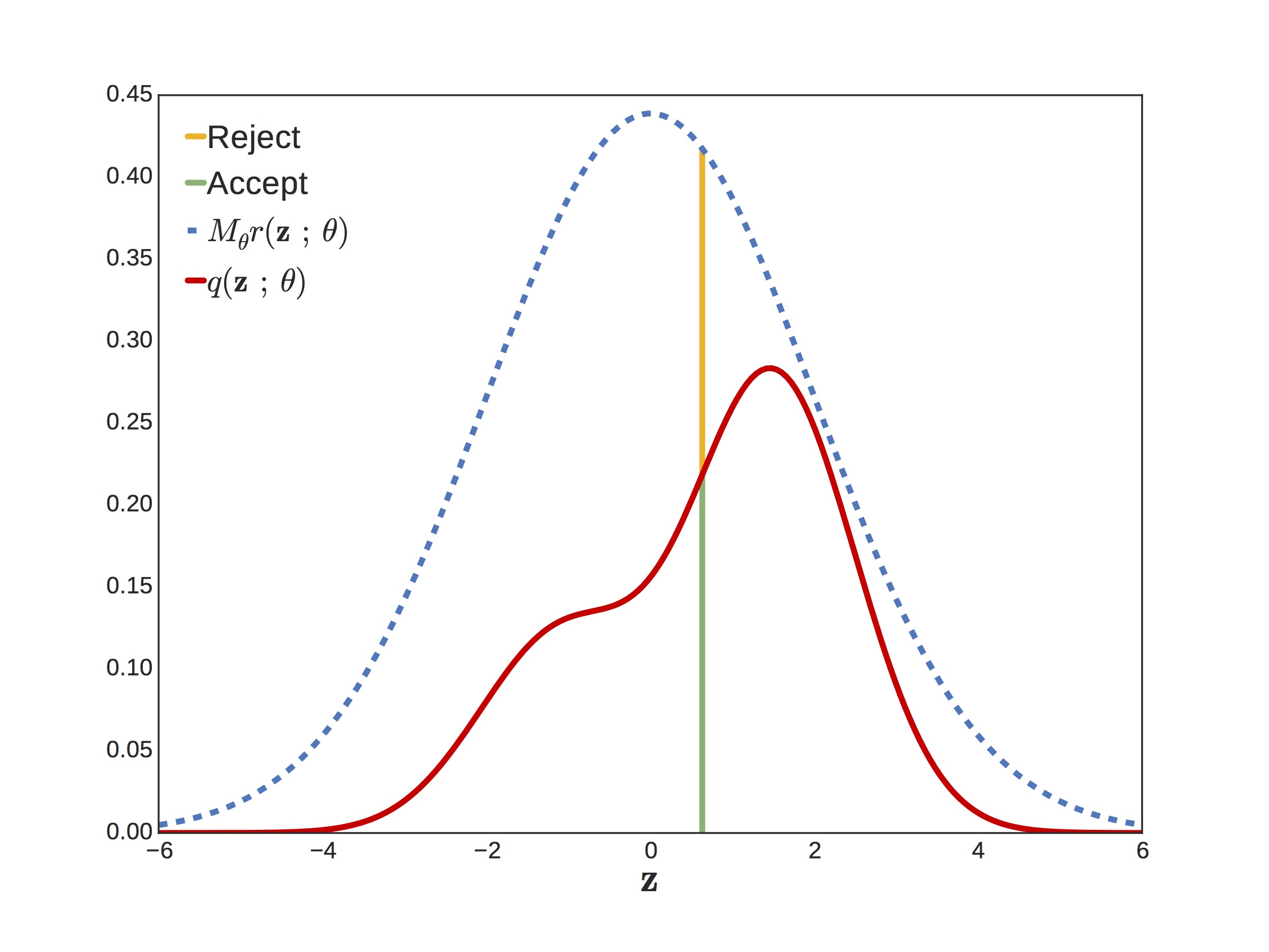
Now put those gradient estimators aside for a minute while we talk about rejection sampling. Suppose you want to sample from a target density $q(z; \theta)$ but it’s too complicated to sample directly. If you can find another density $r(z; \theta)$ and a scaling factor $M_\theta$ such that $M_\theta r(z; \theta) \geq q(z ; \theta) \; \forall z$ , then you can use this as a proposal distribution. For example, in the figure below, the wiggly red curve is our target and the blue curve is our scaled proposal.

The process is super simple. First you draw a sample $z^* \sim r(z; \theta)$ and a uniform value $u \sim \mathcal{U}(0,1)$ . If $u$ is less than the acceptance probability $a(z^*; \theta)$ , you return $z^*$ , otherwise you repeat the process. What is the acceptance probability? It’s just the ratio of the target over the proposal,

$a(z^*; \theta) = \frac{q(z^*; \theta)}{M_\theta r(z^*; \theta)}.$

In the figure below, the acceptance probability is the height of the green over the green plus the yellow. The closer the acceptance probability is to one — i.e. the smaller the gap between proposal and target — the more efficient the rejection sampler.

rejectionsampling

In Python code, a generic rejection sampling algorithm looks like this:

def rejection_sample(sample_r, a, theta):
    while True:
        z = sample_r(theta)
	if npr.rand() <= a(z, theta)):
	    return z

When we presented this at a NIPS workshop, the first question we got was, “Wait, isn’t rejection sampling bad?” The answer is, “No! Well, maybe. It depends.” $^2$ Let me ask you this, is npr.gamma() bad? It uses rejection sampling under the hood, and it turns out that the gamma sampler has an insanely high acceptance probability. On average, its acceptance probability is about 0.95 in the worst case (when the shape is one).

Come to think of it, what is under the hood of npr.gamma()? Numpy, like many other numerical software packages, uses an algorithm by Marsaglia and Tsang [7], which uses as its proposal a simple cubic transformation (which we will leadingly call $h$ ) of a standard Gaussian. For the distribution $\mathrm{Gamma}(\theta, 1)$ with shape $\theta$ and unit scale $^3$ , the Marsaglia and Tsang algorithm uses the proposal,

def h(epsilon, theta):
    # Cubic transform for Ga(theta, 1) proposal
    # Valid only for theta >= 1; for theta < 1,
    # use "shape augmentation" trick mentioned below.
    return (theta - 1./3) * \
           (1 + epsilon / np.sqrt(9*theta - 3))**3
	   
def sample_r(theta):
    # Sample Ga(theta, 1) proposal
    return h(npr.randn(), theta)

The acceptance probability is a bit messier but it just requires a bit of algebra. The key point is that the proposed value of $z$ , and hence the output of the rejection sampling algorithm, is just a transformation of a Gaussian. So why can’t we use the reparameterization trick on gamma random variates?

Rejection Sampling Variational Inference (RSVI)

Let’s recap a bit… First, reparameterization gradients are good because they tend to be low variance. However, it appears that the reparameterization trick is limited to the handful of distributions whose samples can be written as simple transformations of other random variables, which notably excludes the gamma. But wait! The section above showed that the output of the gamma rejection sampler is a simple transformation $z=h(\epsilon; \theta)$ , where $\epsilon$ is a standard normal. The obvious thing to do is to treat the gamma sampling algorithm as a function of $\epsilon$ and apply the reparameterization trick to compute gradients with respect to $\theta$ .

The catch

What is the distribution of $\epsilon$ that we should actually be taking expectations with respect to? It’s not just the standard Gaussian proposal, $s(\epsilon)$ . Recall that the parameters $\theta$ also appear in the acceptance probability! We want the expectation with respect to the distribution of $\epsilon$ that actually lead to an accepted sample of $z$ . Let’s call this density $\pi(\epsilon; \theta)$ . Intuitively, this is just the change of measure of $q(z; \theta)$ under the transformation $z = h(\epsilon; \theta)$ , but we can derive a more general form by marginalizing out the auxiliary acceptance variable as follows,

$\pi(\epsilon; \theta) = \int_0^1 M_\theta s(\epsilon) \mathbb{I}[0 \lt u \leq a(h(\epsilon; \theta); \theta)] \, \mathrm{d} u = M_\theta s(\epsilon) a(h(\epsilon; \theta); \theta).$

Once we have the density of the accepted $\epsilon$ , we want,

$\nabla_\theta \mathbb{E}_{\pi(\epsilon; \theta)} [\log p(x, h(\epsilon; \theta))].$

Unfortunately it seems we are back where we started, with an expectation with respect to a density that depends on the parameters. Sad!

The saving grace

Fortunately, all is not lost. If we expand the expectation we get $^4$ ,

$\nabla_\theta \mathbb{E}_{\pi(\epsilon; \theta)} [\log p(x, h(\epsilon; \theta))] = \int \nabla_\theta \pi(\epsilon; \theta) \log p(x, h(\epsilon; \theta)) \, \mathrm{d} \epsilon.$

Now apply the chain rule and the log derivative trick $^1$ to get,

$\nabla_\theta \mathbb{E}_{\pi(\epsilon; \theta)} = g^{\mathsf{reparam}} + g^{\mathsf{score}}$

where

$g^{\mathsf{reparam}} = \, \mathbb{E}_{\pi(\epsilon; \theta)}[\nabla_\theta \log p(x, h(\epsilon; \theta))],$ $g^{\mathsf{score}} = \, \mathbb{E}_{\pi(\epsilon; \theta)}[\log p(x, h(\epsilon; \theta)) \nabla_{\theta} \log \pi(\epsilon; \theta)].$

In other words, the gradient is the sum of a reparameterization component and a score function component. This is the same form identified by Ruiz et al. [9] in their paper on generalized reparameterizations.

Consider two limiting cases. If the proposal is independent of the parameters — i.e. if $h$ doesn’t depend on $\theta$ — then we reduce to the score function gradient. In the other extreme, when the proposal equals the target then $a(z; \theta) \equiv 1$ , $M_\theta = 1$ , and $\pi(\epsilon; \theta) = s(\epsilon)$ is independent of $\theta$ . Then we reduce to the standard reparameterization gradient. In short, we interpolate between score function and reparameterization gradients as the proposal becomes more and more accurate.

The case of the gamma

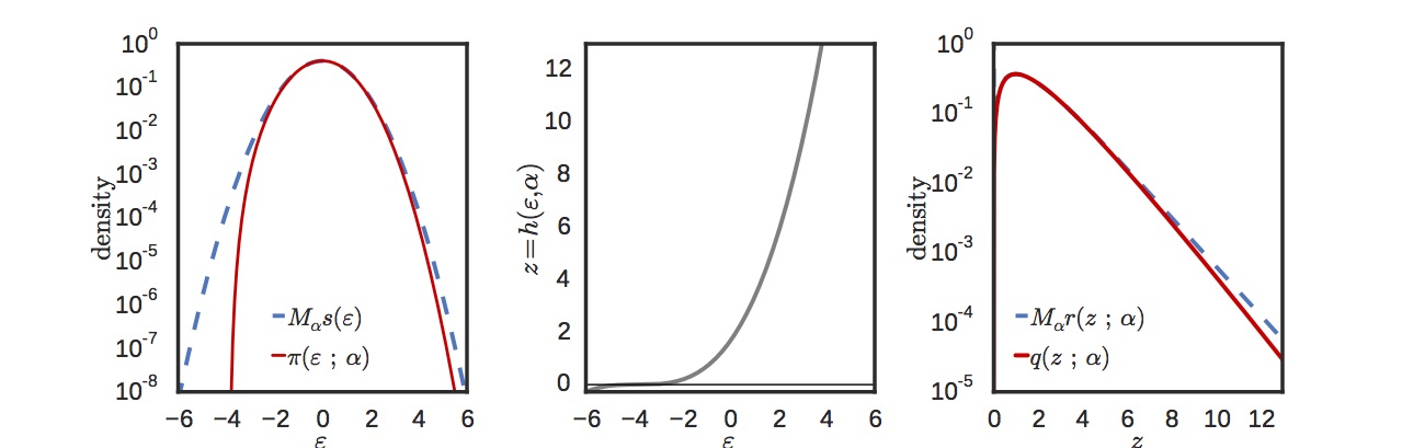
As we remarked earlier, the gamma distribution is used all over the place, and the default way of generating gamma random variates is via rejection sampling. Fortunately, it has a very efficient rejection sampler that uses a cubic transformation of a Gaussian. The figure below shows the log density in $\epsilon$ -space (left) and in $z$ -space (right). The target density is in red and the proposal in blue. For most of the range, the match is extremely accurate. The cubic transformation $h$ is shown in the middle plot.

gamma example

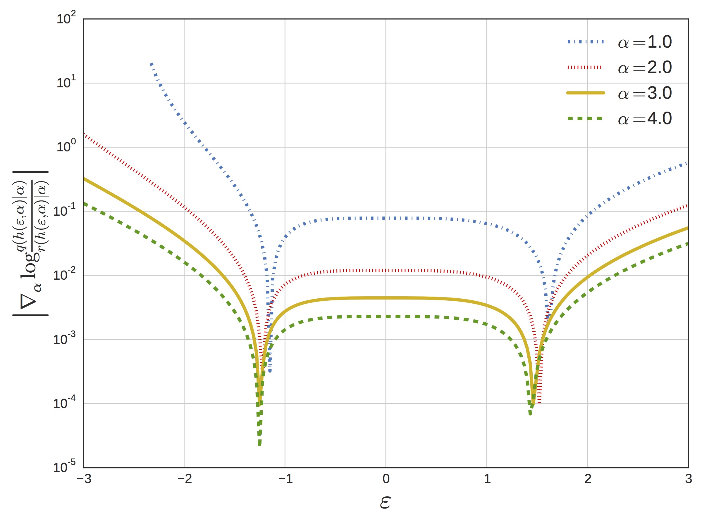
The close match between target and proposal results in a minimal $g^{\mathsf{score}}$ term. We plot this in the next figure, which shows the magnitude of $\nabla_{\theta} \log \pi(\epsilon; \theta)$ (which appears in the definition of $g^{\mathsf{score}}$ ) as a function of $\epsilon$ for a range of different shape parameters.

gamma correction

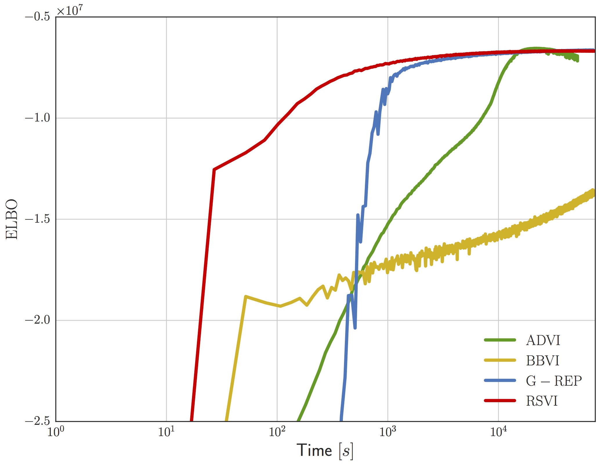
The upshot of all this is that for the gamma distribution we effectively have a complete reparameterization in terms of a standard normal, and this gives rise to much more efficient convergence of the ELBO on real problems. For example, the following figure shows the ELBO as a function of wall-clock time for a sparse gamma deep exponential family (DEF) [8]. We compare against the generalized reparameterization method [9], which is similar to RSVI with a different choice of $\pi(\epsilon; \theta)$ and $h(\epsilon; \theta)$ ; automatic differentiation variational inference [10], which uses a Gaussian variational distribution on $\log z$ ; and black box variational inference [6], which uses the score-function gradient.

sparse gamma DEF

We don’t have space to talk about it here, but our paper goes into detail on an idea we call shape augmentation for working with gamma distributions with shape less than one. Briefly, we can shrink the magnitude of the score function at the expense of doing Monte Carlo over an extended space. In practice, the variance incurred by augmenting the space is well worth it.

Conclusion

Once the gamma is in your toolkit of “reparameterizable” distributions, you immediately get a number of other distributions for free. In particular, the beta and Dirichlet can be obtained by normalizing a set of independently sampled gammas. With RSVI, these fall under the purview of reparameterization. Likewise, the Student’s t distribution can be sampled by generating a gamma and a standard normal, making it immediately amenable to reparameterization. The list doesn’t stop there… the von Mises-Fisher distribution and many others can also be sampled by generating gamma random variates in the inner loop. Luc Devroye’s book [11] contains a treasure trove of sampling methods, many of which use rejection sampling and the gamma distribution as building blocks.

We began with the intuition that all variables sampled in our numerical packages ultimately arise from a deterministic transformation of uniforms, which suggests that we can “reparameterize” much more than initially suspected. Through our study of rejection sampling algorithms, we arrived at a more nuanced view. Namely, we found that care must be taken when this transformation is non-differentiable. Still, in some cases we are able to analytically sum over the discrete choices (e.g. the accept/reject variables or the class assignment in mixture models, as Miller et al [12] do) to obtain a differentiable transformation that we can work with instead.

Where else might this apply? A number of ideas come to mind: what about other Monte Carlo methods, or the accept/reject step in Metropolis-Hastings and HMC? Rejection sampling also appears in a number of discrete sampling methods, like thinning for Poisson processes. Perhaps these methods are useful in those cases as well. It seems we have just scratched the surface of bringing gradient-based methods to bear on partially reparameterizable variational objectives.

Code

Check out some simple code for reparameterizing the gamma distribution in this Jupyter notebook. Full code to generate the figures in the paper is in this repo as well.

Footnotes

This follows from the fact that $\nabla_\theta q(z; \theta) = q(z; \theta) \nabla_\theta \log q(z; \theta)$ .
Given the negative connotation of rejection sampling we decided to rename our paper to use acceptance-rejection sampling instead.
To sample $\mathrm{Gamma}(\theta, \nu)$ you can sample $\mathrm{Gamma}(\theta, 1)$ and divide the returned value by the scale, $\nu$ .
Smoothness of $h$ and $\log p$ are sufficient conditions to move the gradient inside the interval.

References

[1] Naesseth, Christian, et al. “Reparameterization Gradients through Acceptance-Rejection Sampling Algorithms.” Artificial Intelligence and Statistics (AISTATS). 2017. link

[2] Kingma, Diederik P., and Max Welling. “Auto-encoding variational bayes.” arXiv preprint arXiv:1312.6114 (2013). link

[3] Moreno, Alexander, et al. “Automatic Variational ABC.” arXiv preprint arXiv:1606.08549 (2016). link

[4] Srivastava, Akash, and Charles Sutton. “Autoencoding Variational Inference For Topic Models.” International Conference on Learning Representations (2017). link

[5] Nalisnick, Eric, and Padhraic Smyth. “Stick-Breaking Variational Autoencoders.” International Conference on Learning Representations (2017). link

[6] Ranganath, Rajesh, Sean Gerrish, and David Blei. “Black box variational inference.” Artificial Intelligence and Statistics. 2014. link

[7] Marsaglia, George, and Wai Wan Tsang. “A simple method for generating gamma variables.” ACM Transactions on Mathematical Software (TOMS) 26.3 (2000): 363-372. link

[8] Ranganath, Rajesh, et al. “Deep exponential families.” Artificial Intelligence and Statistics. 2015. link

[9] Ruiz, Francisco R., Michalis Titsias RC AUEB, and David Blei. “The generalized reparameterization gradient.” Advances in Neural Information Processing Systems. 2016. link

[10] Kucukelbir, Alp, et al. “Automatic Differentiation Variational Inference.” Journal of Machine Learning Research 18.14 (2017): 1-45. link

[11] Devroye, Luc. Non-Uniform Random Variate Generation. Springer Science & Business Media, 2013. link

[12] Miller, Andrew C., Nicholas Foti, and Ryan P. Adams. “Variational Boosting: Iteratively Refining Posterior Approximations.” arXiv preprint arXiv:1611.06585 (2016). link

Columbia Advanced Machine Learning Seminar

Reparameterization Gradients through Rejection Sampling Algorithms