A few weeks ago we read and discussed two papers extending the Variational Autoencoder (VAE) framework: “Importance Weighted Autoencoders” (Burda et al. 2016) and “Adversarial Autoencoders” (Makhzani et al. 2016). The former proposes a tighter lower bound on the marginal log-likelihood than the variational lower bound optimized by standard variational autoencoders. The latter replaces the KL divergence term — between the approximate posterior and prior distributions over latent codes — in the variational lower bound with a generative adversarial network (GAN) that encourages the aggregated posterior to match the prior distribution. In doing so, both extensions aim to improve the standard VAE’s ability to model in complex posterior distributions.

The figures and tables below are copied from the aforementioned papers.

Variational Autoencoders (VAEs)

The VAE was proposed by Kingma and Welling [3] to perform approximate inference in latent variable models with intractable posterior distributions. The framework trains an encoder —typically a deep neural network— to learn a non-linear mapping between the data space and a distribution over latent variables that approximates the intractable posterior. Simultaneously, a decoder learns a mapping from the latent space to distributions over possible data by estimating the parameters of the data generating process via maximum likelihood .

The Variational Objective

Consider observing a data set $\mathcal{D}=\{x_i\}_{i=1}^N$ where each $x_i$ is sampled iid from a generative process $p(x | \theta)$ involving unobserved latent variables $z$. Formally we write the marginal likelihood

where we suppress the universal dependence on the global parameters $\theta$ for notational convenience. Letting $p_{\mathcal{D}}(x)$ denote the empirical distribution over observed data, the maximum likelihood estimate of $\theta$ is obtained by maximizing $\mathbb{E}_{p_{\mathcal{D}}} \log p(x)$.

However, the marginal likelihood $p(x)$ and posterior distribution over latent variables $p(z \vert x)$ may be computationally intractable, because the conditional density $p(x \vert z)$ may model a complicated non-linear interaction. As such, we would like to form an approximation $q(z\vert x)$ within a tractable parametric family such that

Even with such an approximation, optimizing the marginal likelihood directly may still be intractable. Therefore, we instead optimize the variational lower bound $\mathcal{L}(x)$ obtained via Jensen’s Inequality

Hence, the variational objective may be written as

Reparameterization Trick

In order to efficiently optimize the variational objective we require low-variance, unbiased estimates of the variational lower bound’s gradients. An effective strategy is to introduce auxilliary random variables with a fixed distribution $\epsilon \sim p(\epsilon)$ that is easy to sample from. Then, we may relate the latent variables to the auxilliary variables through a deterministic function $z = g(\epsilon, x, \phi)$ so that

By drawing $k$ iid samples $\epsilon^{(1)}, \cdots, \epsilon^{(k)}\sim p(\epsilon)$ from the auxilliary distribution, we may approximate the gradients of the vartional lower bound with the unbiased Monte Carlo estimator

To make the aforementioned computations tractable AND expressive, the approximating distribution is typically chosen to be approximately factorial with parameters determined by a non-linear function of the data and variational parameters. A common example is a Gaussian distribution with diagonal covariance, i.e.

where the mean and covariance functions $\mu(x, \phi),\Sigma(x,\phi)$ are implemented by a feed-forward neural network and $\epsilon \sim \mathcal{N}(0,I)$. When the generative process $p(x \vert z)$ is similarly implemented by a neural network, the model may be interpreted as a probabilistic auto-encoder with encoder $q(z \vert x)$ and decoder $p(x \vert z)$ (here $\phi$ and $\theta$ represent the parameters of the MLPs); hence the name VAE.

Interpretation

Viewed as an auto-encoder, the VAE attempts to learns an encoder $q(z\vert x)$ that matches the aggregated posterior $q(z) = \mathbb{E}_{p_{\mathcal{D}}}q(z \vert x)$ to the prior $p(z)$ while preserving enough structure so that the decoder $p(x\vert z)$ may generate likely samples. This can be seen by rewriting the objective in its equivalent form

where it becomes clear that a tradeoff is imposed during optimization. The first term penalizes reconstruction error — coercing the encoder and decoder to jointly preserve the structure of the data distribution $p_{\mathcal{D}}$– while the second regularizes the approximate posterior —coercing the encoder to learn a distribution over latent codes similar to the prior $p(z)$.

Importance Weighted Autoencoders

While VAEs are powerful tools for approximate posterior inference, they are limited by the strong assumptions they place on the posterior distrubtion. When these assumptions are not met, they constrain the model into learning an oversimplified representation — one that is approximately factorial with parameters estimable via non-linear regression on the observed data. Moreover, the variational objective over-penalizes the encoder for generating latent samples unlikely to explain the data. Together, these restrictions limit the expressive power of VAEs, which have been empirically observed to underutilize the modeling capactiy of their networks. In order to relieve these constraints, Burda et al. introduce the importance weighted autoencoder (IWAE) which uses an importance sampling strategy to increase the model’s flexibility.

A Tighter Log-Likelihood Lower Bound

Motivated by this intuition, Burda et al. propose a new lower bound on the marginal likelihood

from which it is clear to see that $\mathcal{L}_k(x) \rightarrow \log p(x)$. Moreover, they prove that

showing that the new bound dominates the variational lower bound (noting that the $\mathcal{L}_k(x)$ reduces to $\mathcal{L}(x)$ when $k=1$) and gets tighter with increasing $k$.

Using the reparameterization trick, the Monte Carlo estimator of the gradients of $\mathcal{L}_k(x)$ takes the form of an importance weighted average. To see this, define

to be the raw importance weights and $\tilde{w}_i = w_i / \sum_{j=1}^k w_j$ their normalized counterparts. Now, the estimate

is an importance weighted average of single-sample estimates of the gradient of $\mathcal{L}(x)$ (and as such reduces to the vanilla VAE update rule when the weighted average is replaced with a fair average).

Interpretation

The standard VAE gradient estimates may also be expressed in terms of the importance weights

Noting that the terms $w_i$ exclusively appear inside of the logarithm, we may consider the behavior of the new estimator in terms of the log-transformed importance weights $l_i = \log w_i$. Hence,

where $\psi$ is the well known softmax function. Hence, for large $k$ the importance weighted average

will be dominated by the $\nabla_{\phi,\theta} l_i$ whose generated samples are most likely to explain the data. In this way, we view the importance weighted Monte Carlo estimator as constructing a gradient based on primarily on the “best” samples among $(z^{(1)},\cdots, z^{(k)})$. Consequently, the approximate posterior is encouraged to spread out over the modes of the true posterior, because it is not as harshly penalized for generating occasional samples that are unlikely to explain the data. As such, the IWAE should yield a more expressive model capable of learning higher-dimensional latent representations of the data.

Experiments

To demonstrate the IWAEs increased modeling capacity, its performance was compared to the VAE on density estimation benchmarks. Specifically, multiple configurations of each model were trained on the MNIST and Omniglot datasets and the held-out negative log likelihoods are reported below.

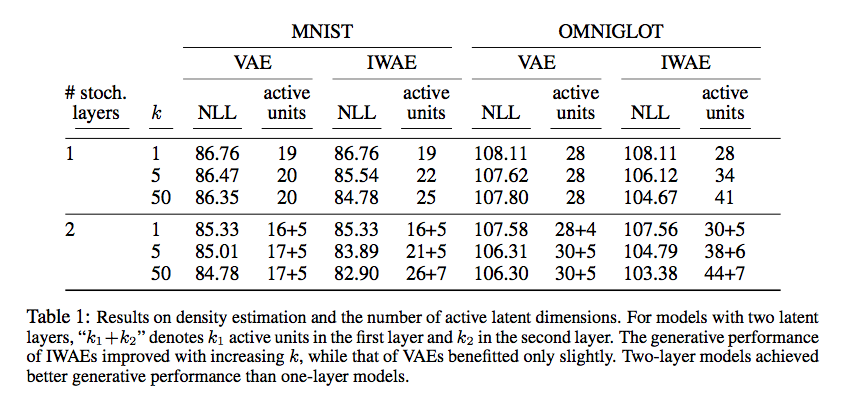
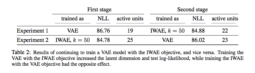
The IWAE outperforms the VAE relative to this metric. Also shown above, the IWAE demonstrates a significant increase in the number of “active units” used while performing these tasks. This metric was proposed by the authors as a way to measure the dimensionality of the learned latent representation. To investigate this property further, an autoencoder was trained using the VAE objective and evaluated on held out data. Following evaluation, training was continued with the IWAE objective and the model was re-evaluated. The reverse experiment was also performed, and the results (below) suggest that replacing the VAE with the IWAE objective increases both the held-out log-likelihood and active units.

Adversarial Autoencoders (AAEs)

While the IWAE objective was derived from a principled lower bound on the marginal likelihood, intuition and heuristics have lead to the development of other VAE variants. Makhanzi et al. [4] proposed the AAE, which replaces the KL regularization term $\mathbb{E}_{p_{\mathcal{D}}}\Big[KL\big(q(z \vert x)\| p(z)\big)\Big]$ in the VAE objective function with a generative adversarial network (GAN) that matches the aggregated posterior $q(z)$ to the prior distribution $p(z)$. In this framework, evaluating the density of the approximate posterior and prior distributions is no longer neccessary so long as one can generate samples from each. In this way, the AAE permits the use of arbitrarily complex, black-box approximating distributions. In addition, the GAN’s discriminator appears to impose stronger regularization on the aggregated posterior, making it match the imposed prior more closely. Together, these changes make the AAE ideally better to image generation: the expressive inference model improves image sharpness, while samples generated by the prior are more likely to yield meaningful images.

Note: The rest of this post assume that the reader has a high-level understanding of GANs. Rather than develop the background here, I urge the unfamiliar reader to check out the review in Robin’s recent post on Modified GANs.

Dual Objectives

The way in which the VAE and GAN architectures are merged is best understood through the following block diagram:

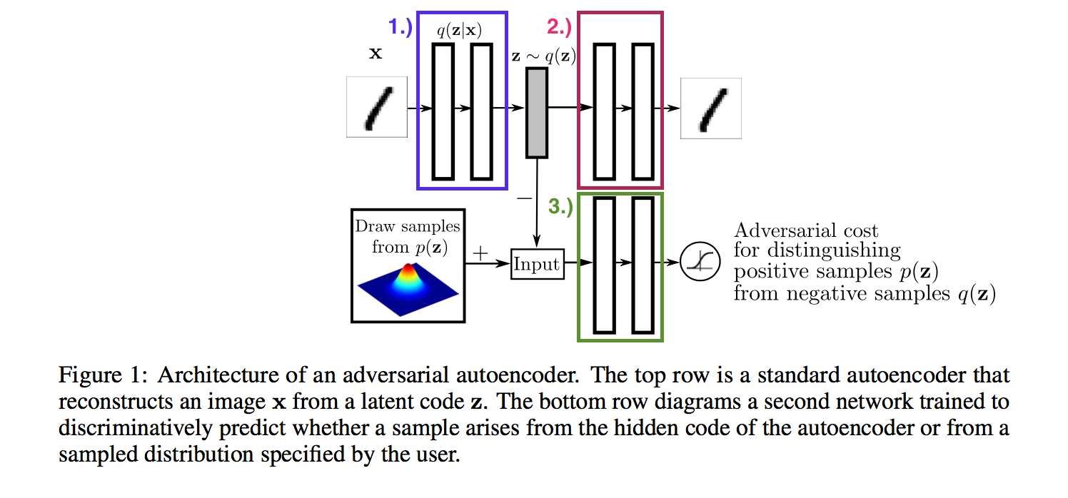
1. $q(z \vert x)$ & $G(x)$: The encoder from the VAE framework is also the generator of the GAN framework.
2. $p(x\vert z)$: The decoder from the VAE framework.
3. $D(z)$: The discriminator of the GAN framework.

Note that the GAN framework has been flipped on its head, so it is worth emphasizing:

• The generator $G(x)$ takes as input data from $p_{\mathcal{D}}(x)$ and produces latent variables $z$ as output.
• The discriminator $D(z)$ distringuishes between latent variables sampled from the aggregated posterior (i.e. corresponding to encoded data) and prior distributions.

It is also worth pointing out that the decoder is unrelated to the GAN framework, so it can be learned via non-linear regression as usual.

The dual objectives are jointly optimized via stochastic gradient descent with two update phases in each iteration:

• Reconstruction Phase: The encoder (generator) and decoder are updated in order to maximize the negative reconstruction error $\mathbb{E}_{p_{\mathcal{D}}}\Big[ \mathbb{E}_{q(z\vert x)}\log p(x\vert z)\Big]$. The reparameterization trick yields the gradient estimator:

• Regularization Phase: The encoder (generator) and discriminator are updated as in ordinary GANs.

Experiments & Applications

To understand how the GAN regularization of the AAE compares to the KL regularization of the VAE, the authors train each on the MNIST dataset and plot the aggregated posterior over hold-out images below.

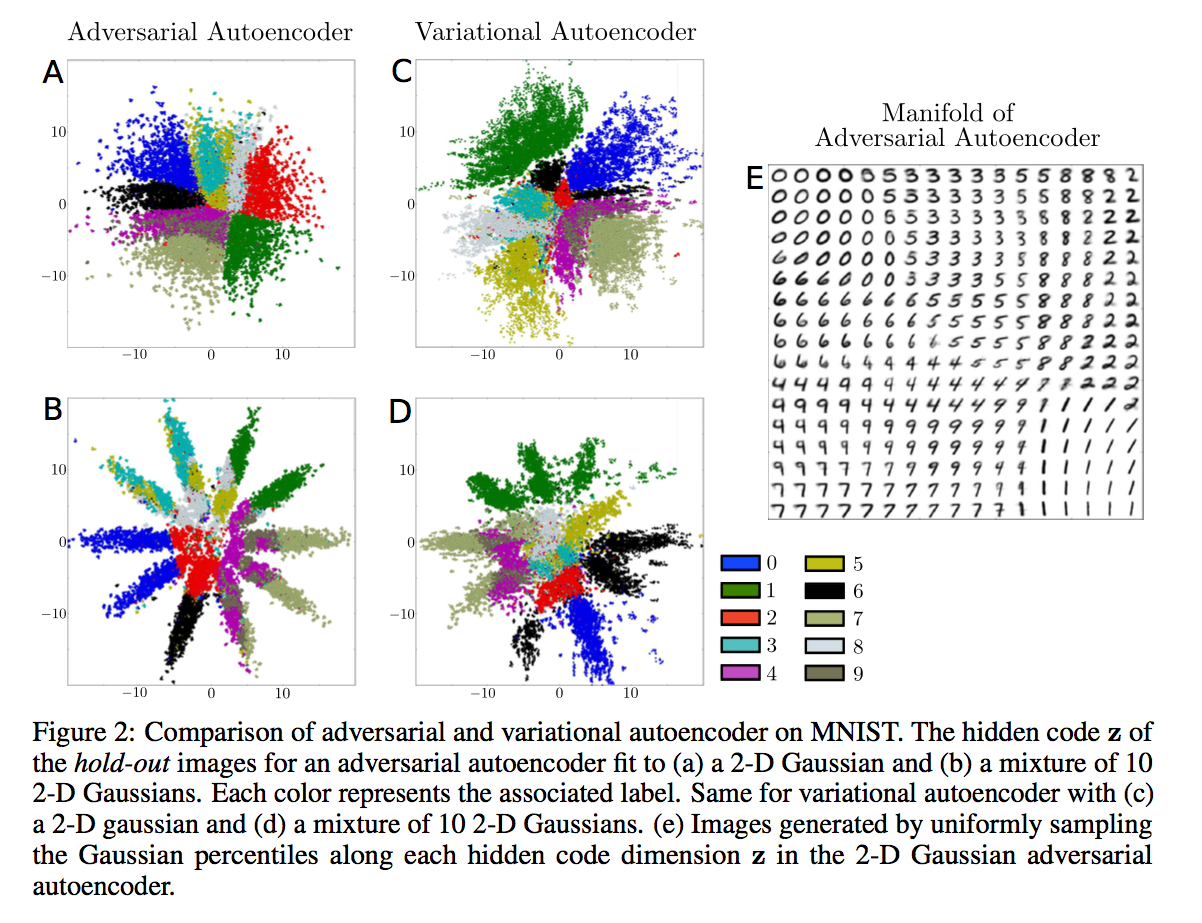
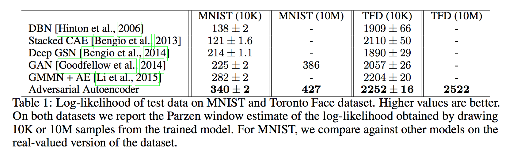
Note that both posteriors resemble the prior, but the AAE provides a much tighter match. The sharp transitions between contiguous regions is desirable for image generation, because samples from the prior are more likely to be mapped to meaningful images and interpolating in the latent space will not yield a latent code outside of the data manifold. Additionally, the authors quantify the improvements afforded by the AAE by evaluating the log-likelihood of held-out validation data after training on the MNIST and Toronto Face datasets. The results are reported below and show substantial improvement over other state-of-the-art methods.

Besides handling the unsupervised learning case, the authors propose a number of modified architectures to handle other learning scenarios. Diagrams of the architectures can be found in [4] and experimetal results demonstrating the performance of each are outlined in the following sections.

Supervised Learning

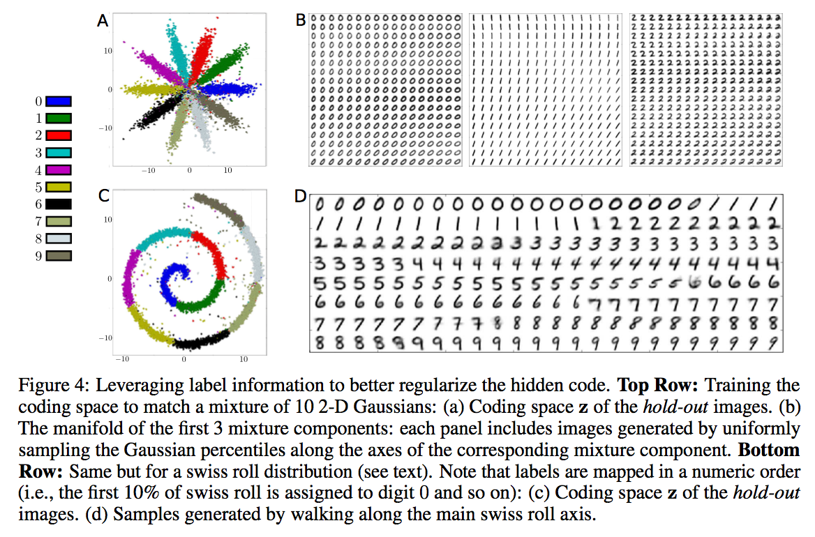
Label information may be leveraged by providing a one-hot vector of class indicators to the discriminator along with the latent code $z$. In this way, the prior distribution may be subdivided or composed of multiple components with each region/component corresponding to a particular label. When used as a generative model, the AAE may then generate new data belonging to particular class by sampling latent codes from the appropriate region/component of the prior. This approach is demonstrated below using images from the MNIST dataset.

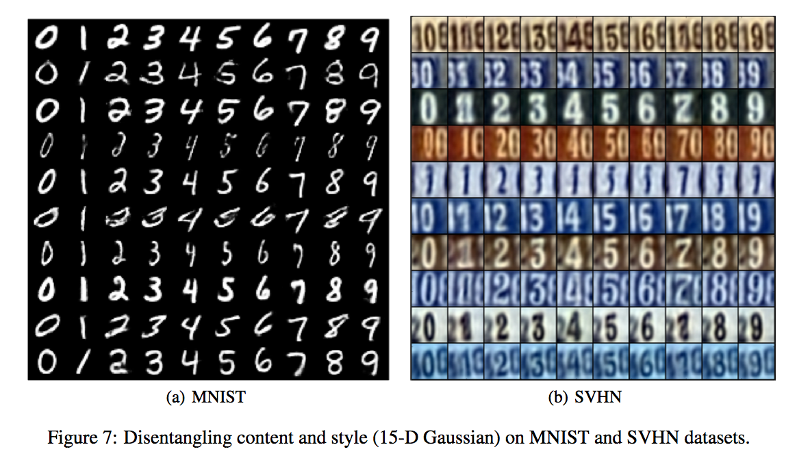
A variant of this method is also introduced in which the label information is provided as input to the decoder instead of the discriminator. As such, the encoder learns a mapping that solely expresses information about the image style, because it no longer needs to preserve information about the image class in the latent code. This approach to uncoupling label and style information is demonstrated below using images from the MNIST and Street View House Number (SVHN) datasets. The images in each row are generated by varying the class label for a fixed latent code.

Semi-Supervised Classification

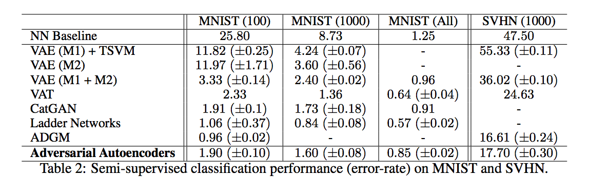
The aforementioned supervised learning algorithms can easily be extended to semi-supervised classification by further modifying the network architecture. The authors propose a solution which replaces the posterior approximation $q(z \vert x)$ with an approximation to the joint posterior over responses and latent codes $q(z,y \vert x)$, adds an additional disciminator which matches the marginal $q(y)$ to a categorical distribution, and introduces a semi-supervised classification phase to the optimization in which the marginal posterior $q(y \vert x)$ is updated with a batch of labeled data. The classification results on the MNIST and SVHN datasets are presented below. Note that while the AAE is outperformed by Ladder Networks and ADGM, it signifcantly outperforms other VAEs.

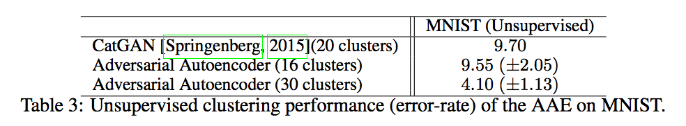
Unsupervised Clustering

An unsupervised clustering framework can be obtained from the previously described semi-supervised classification architecture by ommitting the semi-supervised classification phase. The categorical latent variable $y$ may now be interpretted as an indicator of cluster membership. Below, the authors evaluate clustering performance on the MNIST dataset by assigning the label belonging to the validation sample $\hat{x}_i = \arg\max_{x_n} q(y_i \vert x_n)$ to all of the validation points in cluster $i$. The error rates of this classification rule are presented in the following table.

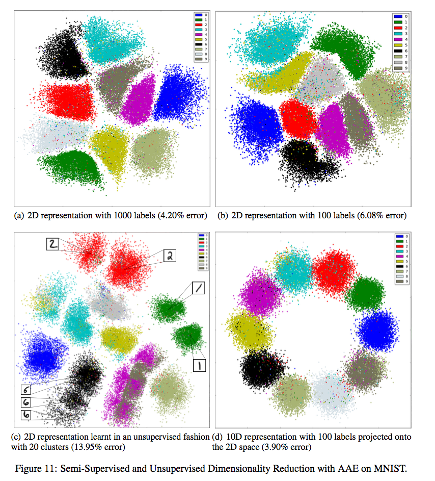
Dimensionality reduction & Visualization

Finally, an AAE variant for dimensionality reduction is introduced by adding yet another modification to the unsupervised clustering architecture. In order to embed the data into an $n$ dimension space, the $m$-dimensional cluster indicator $y$ is mapped to an $n$-dimensional “cluster-head” which is then combined with the $n$-dimensional style code $z$. The sum of these two latent variables yields a final $n$-dimensional representation which is used as input to the decoder. This final representation may also be plotted when $n$ is equal to either $2$ or $3$. The authors use this technique to visualize the MNIST dataset and the embeddings are displayed below.

Recap

Overall, the AAE appears to be a very flexible extension of the VAE which can be extended to perform a number of learning tasks. While the AAE’s dual objective function is motivated primarily by intutiton, it is interesting to note Mescheder et al. [5] derive a very similar algorithm from the variational lower bound and show that the AAE is an approximation to their method. I highly encourage the interested reader to check out that or the post on Modified GANs where it is discussed.

References

[1] Burda, et al. “Importance Weighted Autoencoders.” arXiv preprint arXiv:1509.00519 (2016). link

[2] Goodfellow, et al. “Generative Adversarial Networks.” Advances in Neural Information Processing Systems (2014). link

[3] Kingma & Welling. “Auto-Encoding Variational Bayes.” International Conference on Learning Representations (2014). link

[4] Makhzani, et al. “Adversarial Autoencoders.” arXiv preprint arXiv:1511.05644 (2016). link

[5] Mescheder, et al. “Adversarial Variational Bayes: Unifying Variational Autoencoders and Generative Adversarial Networks.” arXiv preprint arXiv:1701.04722 (2017). link